Assignment Sample on a Regression Model

This page demonstrate the assignment on regression model.

Data can be downloaded from WorldBank Open Data (URL)

Sample R code on Predicting Import 

Assume we would like to predict import value of a country, the dependent variable shall be “import”. Then we can search the variable “import” in the World Bank database. The export data are in the section called trade. The variable we used is title as “Imports of goods and services (current US$)”. Here is the link to the variable (URL=https://data.worldbank.org/indicator/NE.IMP.GNFS.CD)

Since panel data are presented in the World Bank database, however we are only interested in a cross sectional data. Then we choose data of year 2015 as a sample since it is most recent and its completeness.

For explanatory variable, we choose GDP since the trade theories says country will import more when they are richer. GDP will be use as a measurement for the richness of a country. In this case we then use GDP at the current USD price. Here is the link to the variable. (URL=https://data.worldbank.org/indicator/NY.GDP.MKTP.CD)

• Download sample data
• Download R Code (.R file)

# Title: Developing a model to predict export

# 1. IMporting data
mydata <- read.csv("C:/Users/Econ-lab/Desktop/mydata.csv")
<div class="text_exposed_show">
# 2. Descriptive stats
install.packages("psych")
library(psych)

describe(mydata)

# 3. Data viz

# boxplot for normality check
par(mfrow = c(1, 3))

boxplot(mydata$gdp, main ="skew(gdp) = 5.00", col = "darkblue")
boxplot(sqrt(mydata$gdp), main ="skew(sqrt(gdp)) = 2.87", col = "blue")
boxplot(log(mydata$gdp), main ="log(sqrt(gdp)) = 0.14", col = "lightblue")

skew(mydata$gdp)
skew(sqrt(mydata$gdp))
skew(log(mydata$gdp))

# boxplot the import
skew(mydata$import)
skew(sqrt(mydata$import))
skew(log(mydata$import))
par(mfrow = c(1, 3))

boxplot(mydata$gdp, main ="skew(import) = 5.11", col = "darkgreen")
boxplot(sqrt(mydata$gdp), main ="skew(sqrt(import)) = 2.84", col = "green")
boxplot(log(mydata$gdp), main ="log(sqrt(import)) = 0.22", col = "lightgreen")

# plot

plot(mydata$gdp, mydata$export)

plot(log(mydata$gdp), log(mydata$export))

# regression
?lm

model1 &lt;- lm(log(import) ~ log(gdp), data = mydata )
summary(model1)

# log(export) = 1.309 + 0.913log(gdp)
# (0.245) (0.010)
# F-test shows that the model can predict import
# staistically significant at 0.001 level.
#
# R-square = 0.976, gdp can predict 97.6% of variation in import

# plot the result
par(mfrow = c(1, 1))
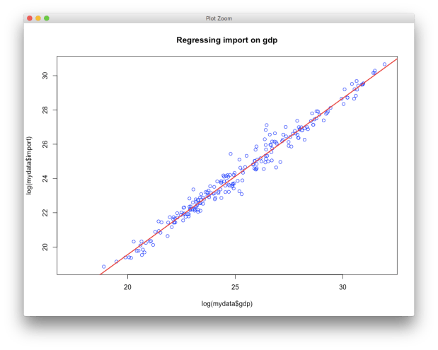
plot(log(mydata$gdp), log(mydata$import))
abline(model1, col = "red", lwd = 2)

Sample output from regression

log(export) = 1.309 + 0.913log(gdp)
(0.245)   (0.010)

Plot a single regression curve over a scatter plot.

# plot the result

par(mfrow = c(1, 1)) # set output window back to a single window

plot(log(mydata$gdp), log(mydata$import)) # scatter plot

abline(model1, col = "red", lwd = 2) # draw a regression line over the plot